Hybrid Image
Hybrid Image
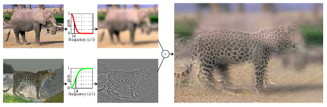
•A. Oliva, A. Torralba, P.G. Schyns, “Hybrid Images,” SIGGRAPH 2006
实验目的
了解图像处理的基础,熟悉高斯滤波操作。
实验原理
根据论文,混合图像是通过在两个不同的空间尺度上叠加两个图像来生成的:低空间尺度是通过低通滤波器对一个图像进行滤波来获得的;通过用高通滤波器对第二图像进行滤波来获得高空间尺度。通过将这两个滤波后的图像相加来合成最终图像。
实验过程
直接高斯滤波
最简单的,我们可以调用OpenCV的GaussianBlur对图像进行高斯滤波,得到低频图像,然后用原图像和减去低频图像就可以得到高频图像。
GaussianBlur函数对操作进行了封装。如
GaussianBlur(low_img, blurred_low, Size(25, 25), 0, 0)生成的高斯滤波器kernel size为25×25,后两个参数为0表示让OpenCV自动根据滤波器大小选择高斯函数中的\(\sigma\)参数。最后面省略了一个参数表示padding的方式,默认为BORDER_DEFAULT,及不含边界值倒序填充。
完整代码如下:
#include <opencv2\opencv.hpp>
#include <iostream>
using namespace std;
using namespace cv;
int main()
{
	Mat high_img;
	Mat low_img;
	high_img = imread("C:/Users/LENOVO/Desktop/CV_course/Einstein.png");
	low_img = imread("C:/Users/LENOVO/Desktop/CV_course/Marilyn.png");
	Mat blurred_low;
	GaussianBlur(low_img, blurred_low, Size(25, 25), 0, 0);
	Mat einstein_mask;
	imshow("blurred", blurred_low);
	Mat highpassed_high;
	GaussianBlur(high_img, highpassed_high, Size(25, 25), 0, 0);
	subtract(high_img, highpassed_high, highpassed_high);
	imshow("highpassed", highpassed_high);
	Mat hybrid_img = blurred_low + highpassed_high;
	imshow("Hybrid Image", hybrid_img);
	waitKey(0);
	return 0;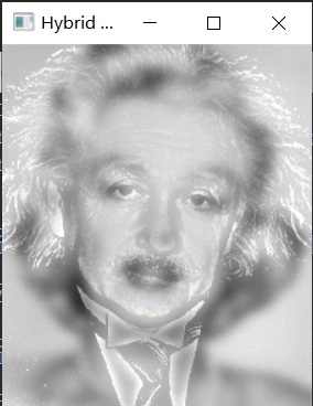
}以经典的Einstein和Marilyn为例得到结果如下所示:
频率域高斯滤波
实际上论文中原文有:
A hybrid image \((H)\) is obtained by combining two images \(\left(I_1\right.\) and \(I_2\) ), one filtered with a low-pass filter \(\left(G_1\right)\) and the second one filtered with a high-pass filter \(\left(1-G_2\right): H=I_1 \cdot G_1+I_2 \cdot\left(1-G_2\right)\), the operations are defined in the Fourier domain. Hybrid images
也就是说我们需要在频率域进行操作。
一张图片可以表示成 \(\sum_{i, j} R_{i j}\), 其中 \(R_{i j}\) 代表作坐标为 \((i, j)\) 的图片像素。
过滤过的图片 \(R\), 是由滤波器 \(H\) 对 \(F\) 做卷积。 \[ \begin{aligned} R_{i j} & =\sum_{u, v} H_{i-u, j-v} F_{u, v} \\ \mathbf{R} & =\mathbf{H} * * \mathbf{F} \end{aligned} \] 与直接高斯滤波不同, \(F\)是将目标图片做过傅立叶转换(FFT),并且将频率零平移置中(FFT Shift) 而产生的2D 频谱(Spectrum) 靠近中央代表低频信号, 靠近边界代表高频信号。其中高频信号代表剧烈或是边角。 其中高斯滤波器 \(H\) 定义如下: \[ g(i, j)=E X P\left(-\frac{(x-i)^2+(y-j)^2}{2 \sigma^2}\right) \] 其中 \(\sigma\)截止频率, \((i, j)\) 是图片像素点位置, 而 \((x, y)\) 是中心点。
下面参照原理动手实现频率域高斯滤波操作。其中这篇文章的python代码给我的整体思路有较大帮助。
output[0] = img.clone();
output[1] = Mat::zeros(img.size(), CV_32FC1);
Mat complexIm;
merge(output, 2, complexIm);
dft(complexIm, complexIm);
// 分离通道(数组分离)
split(complexIm, output);
// 以下的操作是频域迁移
fftshift(output[0], output[1]);
先将原来的图像分成实数域和复数域(暂时为0),再合并通道 (把两个矩阵合并为一个2通道的Mat类容器),进行离散傅里叶变换。
为了方便观察,使用fftshift频域迁移将原点移到中间。OpenCV中没有直接给出fftshift的接口,但实际上它很简单,只是dft取了频谱上$
[ 0 , f s ] $的部分,由于频谱是按 \(\mathrm{f}_{\mathrm{s}}\) 周期延拓,所以
\(\left[\mathrm{f}_{\mathrm{s}} / 2,
\mathrm{f}_{\mathrm{s}}\right]\) 部分的频谱与 \(\left[-\mathrm{f}_{\mathrm{s}} /
2,0\right]\) 部分的一样,如果想看 \(\left[-\mathrm{f}_{\mathrm{s}},
\mathrm{f}_{\mathrm{s}}\right]\) 部分
,就需要做fftshift,将零频分量移到序列中间,对于一维,左右交换即可。图像是二维的,那么就左上和右下交换。
void fftshift(Mat& output0, Mat& output1)
{
	// 以下的操作是移动图像  (零频移到中心)
	int cx = output0.cols / 2;
	int cy = output0.rows / 2;
	Mat part1_r(output0, Rect(0, 0, cx, cy));  // 元素坐标表示为(cx, cy)
	Mat part2_r(output0, Rect(cx, 0, cx, cy));
	Mat part3_r(output0, Rect(0, cy, cx, cy));
	Mat part4_r(output0, Rect(cx, cy, cx, cy));

	Mat temp;
	part1_r.copyTo(temp);  //左上与右下交换位置(实部)
	part4_r.copyTo(part1_r);
	temp.copyTo(part4_r);

	part2_r.copyTo(temp);  //右上与左下交换位置(实部)
	part3_r.copyTo(part2_r);
	temp.copyTo(part3_r);

	Mat part1_i(output1, Rect(0, 0, cx, cy));  //元素坐标(cx,cy)
	Mat part2_i(output1, Rect(cx, 0, cx, cy));
	Mat part3_i(output1, Rect(0, cy, cx, cy));
	Mat part4_i(output1, Rect(cx, cy, cx, cy));

	part1_i.copyTo(temp);  //左上与右下交换位置(虚部)
	part4_i.copyTo(part1_i);
	temp.copyTo(part4_i);

	part2_i.copyTo(temp);  //右上与左下交换位置(虚部)
	part3_i.copyTo(part2_i);
	temp.copyTo(part3_i);
}
之后按照公式进行高斯滤波即可。取高频信号时可以直接将高斯滤波器翻转。
Mat gaussianBlur(test.size(), CV_32FC1); //,CV_32FC1
if (is_high)
{
    for (int i = 0; i < test.rows; i++) {
        for (int j = 0; j < test.cols; j++) {
            float d = pow(float(i - test.rows / 2), 2) + pow(float(j - test.cols / 2), 2);
            gaussianBlur.at<float>(i, j) = 1 - expf(-d / (2 * sigma * sigma));
        }
    }
}
else {
    for (int i = 0; i < test.rows; i++) {
        for (int j = 0; j < test.cols; j++) {
            float d = pow(float(i - test.rows / 2), 2) + pow(float(j - test.cols / 2), 2);
            gaussianBlur.at<float>(i, j) = expf(-d / (2 * sigma * sigma));
        }
    }
}
得到高斯滤波器后对图片进行过滤,实部虚部分别与滤波器模板对应元素相乘。最后还要进行逆变换,归一化,得到最终滤波图像。
Mat blur_r, blur_i, blur_full;
multiply(output[0], gaussianBlur, blur_r);
multiply(output[1], gaussianBlur, blur_i);
Mat blur_split[] = { blur_r, blur_i };
fftshift(blur_split[0], blur_split[1]);
merge(blur_split, 2, blur_full);
idft(blur_full, blur_full);
blur_full = blur_full / blur_full.rows / blur_full.cols; // 归一化
split(blur_full, output);
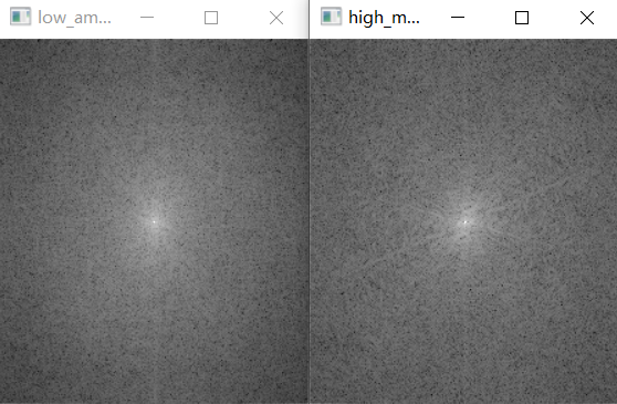
output[0] = output[0] / 255;我们还可以将离散傅里叶变换得到的结果转换成幅值矩阵展示出来:
Mat amplitude;
magnitude(output[0], output[1], amplitude);
amplitude = amplitude + Scalar::all(1);
log(amplitude, amplitude);
normalize(amplitude, amplitude, 0, 1, NORM_MINMAX);
imshow(text, amplitude);
一般来说,低频的信号幅值大,组成一个信号的基本面,高频的信号幅值小,刻画细节、轮廓。
对傅里叶变换及应用的粗浅理解参照了这里。
结果展示
使用OpenCV附带的Trackbar功能实现了自动调节截止频率的功能。展示如下:
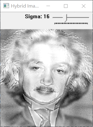
可以看到\(\sigma=16\)时能够取得较好的混合效果。
得到两个图片的幅值矩阵如下所示:
换用自己喜欢的图像尝试一下:
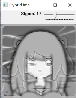
因为这两张图片都不存在明显的高频信号,因此不是一个很好的样例。